In this article we will introduce the context surrounding word2vec, including the motivation for distributed word embeddings, how the Continious Bag-of-Words and Skip-gram algorithms work, and the advancements since the original paper was released. We will also go into the training of the neural network, so it is assumed you have some knowledge on this.

Word2Vec Paper 1- introducing CBOW and Skip-Gram	Word2Vec Paper 2- Performance Improvements

Motivation

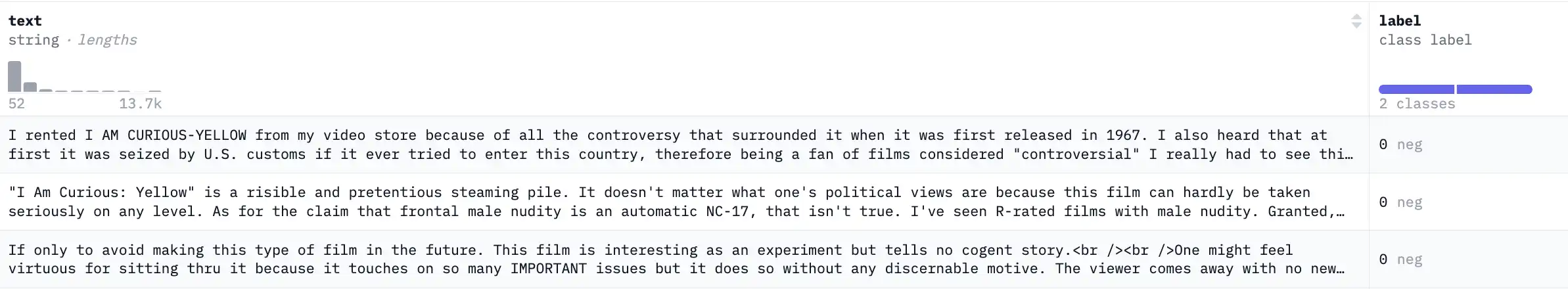
For many NLP tasks, we need to learn on data which can’t be easily represented numerically. For example, let’s look at the popular IMDB dataset, which gives reviews in one column, and a binary sentiment label in the next:

The ‘old’ way:

We can represent a corpus of words using a Bag-of-Words. For some input text, we can create an unordered ‘bag’ of the text’s vocabulary (set of unique words), and how many count times it appears in the text.

Raw text:

"Ogres are like onions, onions have layers.

Bag-of-Words:

{"Ogres": 1, "are": 1, "onions": 2, "like": 1, "have": 1, "layers": 1}

We can use a BOW to represent any word from our corpus using one-hot encoding:

Onions:  [0,0,1,0,0,0]

Ogres: [1,0,0,0,0,0]

Although an ML model could learn using this method, it is grossly inefficient: imagine a corpus with a vocabulary (number of unique words) of 100,000. This would mean you would need a combined vector size of 1,000,000 to encode just 10 words, where 99.9% of the vector is empty.

The ’new’ way:

word2vec creates a distributed representation of words, which is much more efficient, and allows much a much larger corpus of text to be used in training.

Each vector is continious and dense, where vectors that are closer have similar meanings. This distributed representation of a large text corpus is our goal, so we can use it in other NLP tasks, and word2vec is how we will accomplish it. Since 2013, there are better ways to do this, such as BERT and GloVe, which can embed more nuanced relationships between words.

Dense embedding of ‘Ogre’:

array([ 7.10577386e-01, -5.09895974e-01,  1.71235001e+00,  2.05854094e+00, -4.47590043e-01, -1.00782587e+00, -1.14494191e+00, -7.94087996e-01, -2.22047371e-01,...])

array_shape: (400,)

The famous example given in the paper is that using vector math with the final embeddings, you could do something like: $\vec{King} - \vec{Man} + \vec{Woman} = \vec{Queen}$. In reality, the resultant vector may not line up exactly with $\vec{Queen}$, but Queen should be the closest vector using cosine distance.

‘Closeness’: If every word is a vector, ‘closeness’ between any 2 words (vectors) can be defined as a dot-product of those vectors being close to 1.

Distributional similarity- representing a word by means of its neighbors. For a word, its meaning must be encoded by all of the words that are near it in every context. For example, if we look for the word ‘banking’ across a massive corpus of text, and note all the words nearby, these words must somehow encode the meaning of ‘banking’.

How Word2Vec encodes words

Now we understand why we need to encode words as dense vectors that embed meaning, we can jump in to how word2vec accomplishes this. The paper establishes 2 ‘fake’ tasks that get the model to learn embeddings:

Continuous Bag-of-Words (CBOW)

The neural network is passed a few context words from around the target word, with the goal of predicting what that target word is.

Skip-gram

The opposite of CBOW, the model is instead passed the middle word, with the goal of predicting the context words around it.

note: These words will be passed to the model as one-hot encodings

Retrieving embeddings

Softmax activation

Although later word2vec papers go on to describe the more efficient hierarchical softmax, we will focus just on how softmax helps us clarify which word the network is predicting.

$$ \text{Softmax}(x_{i}) = \frac{\exp(x_i)}{\sum_j \exp(x_j)} $$

The softmax activation can take a vector of numbers, and maps each number to between $[0,1]$, where the sum of the vector will always add up to 1. From this, we can find our model’s prediction by getting the element with the highest number.

Training

Using a context window, we can generate pairs for the model in the form: (TARGET,CONTEXT)

Becomes the following pairs:

(onions,ogres), (onions,are), (onions,like), (onions,they), (onions,have), (onions,layers)

And using the next target word:

Becomes these pairs:

(they,ogres), (they,are), (they,like), (they,onions), (they,have), (they,layers)

Using a training pair, $(Y,X)$ (both one-hot encoded), the model will get passed $X$, and have its output compared against $Y$ to learn from.

Distinction between CBOW and Skip-gram training

It’s important to make a distinction regarding these pairs for the 2 models, because they are slightly different:

• For Skip-gram, the model would be passed a target word ($Y$), and for output, predicts all the words within the context window ($ X_{i-n} $). If we had 10 words in the vocabularly, and a context size 3, this would make the model’s output vector shape (6,10)- one row for each context word.
• For CBOW, the model is passed all words in the context window ($X_{i-n}$), and for output, predicts the target word that fits the best ($Y$). Inside the neural network, the projection layer, which maps input to the hidden layer, averages all the word vectors into one, so after this step, the network is working with one average word vector.

That’s just about it! I hope you’ve learned something from this article- in the next one in this series, I will be going through building the word2vec CBOW model in python within numpy.

Sources / Further Reading:

• Chris McCormik- Word2Vec guide

• Word2Vec from scratch with python and numpy

• Jake Tae- Word2Vec from scratch

• Word2Vec original paper